

We will start a series of tutorials regarding the most significant science disciplines and which represent the future of data science which is Machine-Learning and Deep-Learning and here we will start with Machine-Learning.
• What is Machine learning?
• Types of Machine Learning
• Models and Algorithms
• Get the concept of prediction with Simple Machine Learning
What is Machine learning (ML)?
ML is representing a side of Artificial Intelligence (AI) that enables the computer to learn from data and do things that are not programmed to do it explicitly. ML uses a variety of mathematical and statistical operations called “Algorithms” that are responsible for learning a certain model the data have been received. An ML model represents the generated mapping function that represents a map from inputs to outputs. The model could be predictive, classification, clustering model, and so on.

Basic Types of Machine Learning
- Whether or not they are prime with mankind control (supervised, unsupervised, semi-supervised, and Reinforcement Learning)
- Whether or not they can learn incrementally on the fly (online versus batch learning).
- Whether they activity by easy similarly new data points to known data points, or instead suspect layout in the training data and build a predictive model, much like scientists do (instance-based versus model-based learning)
Models and Algorithms
“Model” represents the mapping function that leads inputs to their outputs and this mapping function is trained by the “Algorithm” (some kind of mathematical/statistical operations).
Y=f(X) Y=f(X)
As this mapping function will not lead to the exact right outputs since its job only is trying to get the best performance and mapping between input data and right outputs, which results in some kind of errors so we can modify the above equation to be:
Y=f(X)+eY=f(X)+e
The whole picture will be clear when start handling the first type of Machine-Learning which is Supervised Learning
Supervised learning
In supervised ML, the actual/real output is already known and the whole process is fully under man supervision. This type is divided into two main categories Regression (Continuous data prediction) and Classification (Determine in which class our data belongs to)
Regression
Generalized Linear Models
The general equation for a linear system could be expressed as follows:
𝑦^(𝑤,𝑥) =𝑤0+𝑤1𝑥1+...+𝑤𝑝𝑥𝑝
• where: (𝑦^) is the predicted output.
In (Scikit-Learn) module, coefficients vector 𝑤= (𝑤1…) is expressed as coef_ and 𝑤0 as intercept_
Ordinary Least Squares (OLS)
You can learn more about the effect of variation on coefficients on the regression line by the visualization on http://setosa.io/ev/ordinary-least-squares-regression/
OLS Is the method used by Linear Regression in which the minimum sum of squared errors between predicted and actual output values is a target and its cost function could be expressed as:
β∗0,β∗=argminβ0,β(1n∑i=1n(yi−(x∗iβ+β0))2)β0∗,β∗=argminβ0,β(1n∑i=1n(yi−(xi∗β+β0))2)
Tip: OLS depends on its calculations that model inputs are independent. When model inputs are correlated, which means that there is a possibility of existing some kind of linear relationship between them, which leads in large variance.
import pandas as pd

import numpy as np

import matplotlib.pyplot as plt

%matplotlib inline
# Importing our dataset from CSV file:

dataset = pd.read_csv('./Datasets/student_scores.csv')
# Now let's explore our dataset:

dataset.shape

(25, 2)
# Let's take a look at what our dataset actually looks like:

dataset.head()
| Hours | Scores | |
|---|---|---|
| 0 | 2.5 | 21 |
| 1 | 5.1 | 47 |
| 2 | 3.2 | 27 |
| 3 | 8.5 | 75 |
| 4 | 3.5 | 30 |
# To see statistical details of the dataset, we can use describe ():

dataset.describe()
| Hours | Scores | |
|---|---|---|
| Count | 25.000000 | 25.000000 |
| Mean | 5.012000 | 51.480000 |
| Std | 2.525094 | 25.286887 |
| Min | 1.100000 | 17.000000 |
| 25% | 2.700000 | 30.000000 |
| 50% | 4.800000 | 47.000000 |
| 75% | 7.400000 | 75.000000 |
| Max | 9.200000 | 95.000000 |
Where:
- Count: No. of elements in each feature (column).
- Mean: is the mean value per each specification.
- Std: is standard deviation per each segment.
- Min/max is the minimum and maximum values per each portion.
- 25%/50%/75%: are percentile values.
# Plot the dataset and try to guess the relationship between them
dataset.plot(x=’Hours’, y=’Scores’, style=’^’)
plt.title(‘Student Time/Score Graph’)
plt.xlabel(‘Hours Studied’)
plt.ylabel(‘Gained Score’)
plt.show()
We can notice that, data could be expressed by linear relationship between the hours studied and student score.
In [37]:
# preparing our data:
# Divide the data into "attributes/features/inputs" and "labels/targets/outputs".

X = dataset.iloc[:, :-1].values # all colomns except the last one (reshape it into column vector)

y = dataset.iloc[:, 1].values # first colomn only
In [38]:
'''
Splitting our data into training and test sets.
We'll do this by using Scikit-Learn's built-in train_test_split() method:
'''
from sklearn.model_selection import train_test_split
X_train, X_test, y_train, y_test = train_test_split(X, y, test_size=0.2, random_state=0)

# The above script splits 80% of the data to training set while 20% of the data to test set.
In [39]:
# Training the Our Model using Linear-Regression Algorithm:

from sklearn.linear_model import LinearRegression
regressor = LinearRegression()
regressor.fit(X_train, y_train)
Out[39]:
LinearRegression(copy_X=True, fit_intercept=True, n_jobs=None, normalize=False)
In the theory section, we said that the linear regression model basically finds the best value for the intercept and slope (based on OLS), which results in a line that best fits the data. We can retrieve their values by executing the following code.
In [40]:
# To retrieve the intercept:
print(regressor.intercept_)

# For retrieving the slope (coefficient of x):
print(regressor.coef_)
2.018160041434683
[9.91065648]

This means that for every one unit of change in hours studied, the change in the score is about 9.91%
In [41]:
# Making Predictions:
# Now that we have trained our algorithm, it's time to make some predictions.

y_pred = regressor.predict(X_test)    # predicted values.
In [42]:
# To compare the actual output values for X_test with the predicted values, execute the following script:

df = pd.DataFrame({'Actual': y_test, 'Predicted': y_pred})
df
Out[42]:
| Actual | Predicted | |
|---|---|---|
| 0 | 20 | 16.884145 |
| 1 | 27 | 33.732261 |
| 2 | 69 | 75.357018 |
| 3 | 30 | 26.794801 |
| 4 | 62 | 60.491033 |
In [43]:
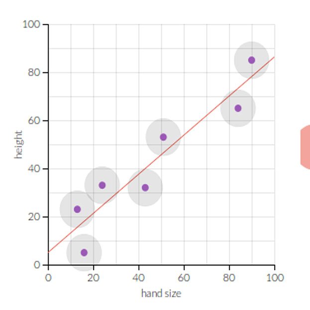
# Plot actual value vs predicted one:
plt.scatter(X_test, y_test)
plt.plot(X_test, y_pred, color='red')
plt.title('Hours vs Percentage')
plt.xlabel('Hours Studied')
plt.ylabel('Percentage Score')
plt.show()
The final step is to evaluate the performance of the algorithm. For regression algorithms, four evaluation metrics are commonly used:
Evaluating the Algorithm:
Mean Absolute Error
MAE=1N∑i=1N|yi−y^i|MAE=1N∑i=1N|yi−y^i|
Mean Squared Error
MSE=1N∑i=1N(yi−y^i)2MSE=1N∑i=1N(yi−y^i)2
# r2_score
R2=1−MSE( model ) MSE (baseline) R2=1−MSE( model ) MSE (baseline)
The MSE of the model is computed as above, while the MSE of the baseline is defined as:
MSE( baseline )=1N∑i=1N(yi−y¯)2MSE( baseline )=1N∑i=1N(yi−y¯)2
In [44]:
from sklearn import metrics
print('Mean Absolute Error:', metrics.mean_absolute_error(y_test, y_pred))
print('Mean Squared Error:', metrics.mean_squared_error(y_test, y_pred))
print('Root Mean Squared Error:', np.sqrt(metrics.mean_squared_error(y_test, y_pred)))
print('r2_score: ', metrics.r2_score(y_test,y_pred))
Mean Absolute Error: 4.183859899002975
Mean Squared Error: 21.5987693072174
Root Mean Squared Error: 4.6474476121003665
r2_score:  0.9454906892105356
You can see that the value of root mean squared error is 4.64, which is less than 10% of the mean value of the percentages of all the students i.e. 51.48. This means that our algorithm did a decent job.
Lower RMSE and higher R-squared values are indicative of a good model. The ideal value of RMSE value is to be close zero-value and for R-squared value is close to 1.


